Open in

Keep Calm and Carry on: A v M in a Wells World

[2026] 2 FRJ 114. This article takes a closer look at how Carry was shared in the cases of A v M and ED v AP, and the different approaches adopted for its assessment. It concludes by proposing an alternative method by which Carry can be shared when the timing of future receipts is unknown.

Introduction

The quantification and valuation of carried interest (or Carry) is often a contentious issue in financial remedy proceedings. This is because Carry is illiquid, uncertain in value and only realisable at some future (and often unknown) point in time. These factors make it difficult to know the value that should be attributed to it. To complicate matters further, Carry can also be highly valuable if certain criteria are met (or entirely valueless, if those criteria are not met), and, as a result, can often be a key asset in the case.

The Family Court has adopted different approaches to deal with Carry, as illustrated by A v M [2021] EWFC 89 (Mostyn J) and, more recently, ED v AP [2025] EWFC 399 (HHJ Hess, sitting as a deputy High Court Judge) and B v B [2013] EWHC 1232 (Fam) (Coleridge J), before that.

In this article, we take a closer look at how Carry was shared in the cases of A v M and ED v AP, and the different approaches adopted for its assessment. We conclude by proposing an alternative method by which Carry can be shared when the timing of future receipts is unknown. This method maintains the simplicity of Mostyn J’s ‘formulaic’ approach, but also accommodates the passing of time (and the work undertaken in that period) as reflected in HHJ Hess’ ‘tapered’ approach.

We also provide a Microsoft Excel tool to enable practitioners to calculate the marital sharing percentage under this approach, as well as vary the assumptions contained in the A v M Formula, where appropriate.[[1]]

Carry and the case for Wells sharing

Carry is a form of compensation that is sometimes earned by individuals working in finance and investment businesses.[[2]] In simple terms, an entitlement to Carry represents the allocation to an employee (who, for ease, we will refer to as the ‘Carry Owner’) of a share of the investment returns earned by the investment firm. Those investment returns are, most typically, generated from amounts invested via a ‘Fund’ structure. The receipt of Carry is often predicated on the returns (i.e. profit) of the Fund surpassing a given rate of return (sometimes referred to as a ‘Hurdle Rate’). These Funds can span many years, with Carry typically only being paid out once the investments made are disposed of, often many years into the future.

As a result, and in the context financial remedy proceedings, the consideration of Carry can raise two distinct computation problems. These are:

(1) How to quantify the value of Carry, where its value may be uncertain and unknowable during the proceedings, as it is dependent on the future performance of the underlying investments held by the Fund; and

(2) How to determine the marital proportion of Carry, given that the timing of Carry payments to the Carry Owner are similarly uncertain and unknowable, as they depend on either the timing of the disposal of the Fund’s underlying investments or the end of the life of the Fund.

Problem (1) – how to deal with an uncertain and unknowable future receipt – already appears to have been answered by the court, namely by way of so-called Wells sharing. For example, in ED v AP (at [57]), HHJ Hess explained that, whilst Wells sharing arrangements are typically undesirable in family proceedings, he nonetheless agreed with Lewison LJ in Versteegh v Versteegh [2018] EWCA Civ 1050 (at [135]) that in cases involving large amounts of contingent assets, such as Carry, Wells sharing can be necessary to avoid ‘considerable unfairness’. He therefore proceeded to adopt this approach when considering how Carry should be quantified in that instance.

But what about Problem (2)? If Carry is to be Wells shared, is there a method that allows the appropriate marital percentage to be assessed given that the issue of the timing of receipt is equally uncertain and unknowable? The cases of A v M and ED v AP are instructive in terms of the different way the courts can approach this issue.

The A v M Formula

In A v M, Mostyn J assessed the marital (and thus shareable) proportion of the husband’s Carry using the following formula (the ‘A v M Formula’):

A/B = C

Where:

A is the period between the establishment of the Fund and the date of the trial;

B is the expected life of the Fund; and

C is the resulting marital proportion to be shared by the parties.

In adopting the A v M Formula, Mostyn J sought to determine the marital share of the value of the husband’s Carry in two funds. In that case, he reallocated the wife’s share of the husband’s Carry in a latter, second fund to an earlier fund, after adjusting for the relative projected future values of Carry for each. That is, Mostyn J concluded that the wife should receive an enhanced share of the husband’s Carry in the earlier fund when realised (and no share of the latter fund).

In the recent judgment of ED v AP (at [58(v)]), HHJ Hess outlined what he considered to be two primary concerns with the A v M Formula, namely that:

(1) it relies upon an unreliable estimate of the end date of the Fund to determine the end date of ‘B’; and

(2) it assumes that work on the Fund occurs linearly across its lifetime, which is not always the case (and which HHJ Hess considered to be an unreasonable assumption in ED v AP).

As a consequence of these issues, HHJ Hess moved away from the strict mathematical and formulaic approach of the A v M Formula. Instead, he adopted alternative sharing percentages for the Carry arising from the different Funds in the case, each of which were established at different times and therefore spanned different periods of the marriage.

In doing so, HHJ Hess concluded, in a holistic manner, that the Funds which spanned the longest periods of the marriage should be shared to a greater extent, as compared to the Funds which straddled smaller portions of the marriage, which should be shared to a lesser percentage.

In our view, however, in both of A v M and ED v AP, one drawback arises. By fixing the sharing percentage at a given point in time (i.e. at final hearing), the marital element is effectively ‘locked in’, even though the precise timing of the Carry payout is unknown and unknowable. What this means is that if investments held by the Fund are realised earlier than was anticipated at the time of the final hearing, the post-marital endeavour can be overestimated, and therefore the marital proportion underestimated. Conversely, if investments are realised later than anticipated, the post-marital endeavour can be underestimated, and therefore the marital proportion overestimated.

To put it another way, in order to determine the precise marital proportion to be shared at the date of trial, even where the ultimate proceeds are to be Wells shared, the court has, up till now, relied on an uncertain estimate of when the Carry might be received.

In the authors’ eyes, this has the appearance of being somewhat inconsistent; why (rightly, we suggest) make provision for the uncertainty of the quantum of the Carry (by way of Wells sharing) but not the uncertainty of the marital element? Both quantum and marital element are unknowable, why not apply the same Wells sharing logic to both?

In the following section, we propose an extension of the time apportionment principles developed by Mostyn J and the A v M Formula to accommodate variable future dates of Carry receipt. Whilst, for ease, we refer to this proposed, new approach as A v M (Extended), we should emphasise it is really just a broader application of the A v M Formula itself.

A v M in a Wells world

In summary, the authors propose extending the A v M Formula to enable the marital proportion of a Carry receipt to be dependent on the date that it is actually received, rather than an estimate at trial of when it might be received. Explicitly, we propose adopting a flexible, formulaic approach that tweaks the A v M Formula so that the end date of ‘B’ is determined at a later date, once it is known with certainty, i.e. once Carry has been received (or is receivable).

The result is that both computational problems, i.e. Problems (1) and (2) above (the quantum of Carry and its marital proportion) are variable, but assessed accurately, only once the relevant parameters are known. In effect, this adopts Wells sharing for the quantum and the analytical equivalent for assessing the marital proportion (i.e. A v M (Extended)).

By way of illustration, in Figure 1 we show how, using the A v M (Extended) approach, the marital proportion of Carry would change over time based on adopting alternative end dates of ‘B’ for when the Carry is actually received. For example:

(1) If the Carry was received on the date of final hearing, then the A v M (Extended) methodology would treat all work to get to that point as marital, and thus the proceeds would be shared equally.

(2) Conversely, as the date of receipt of Carry extends further into the future and beyond the end of the marriage, a greater proportion of work would be treated as non-marital and thus the sharing percentage would be reduced.

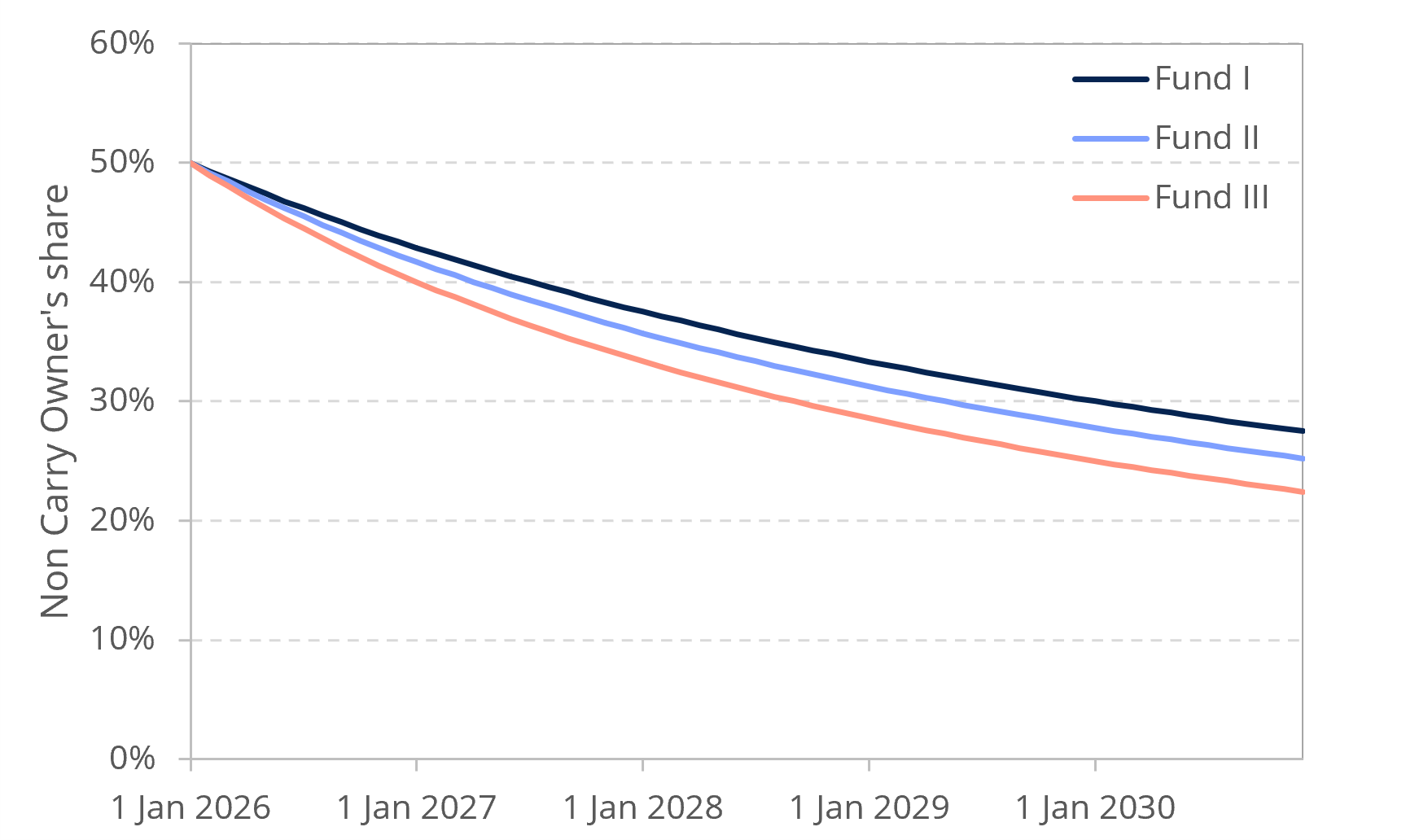
Figure 1: Illustrative example of the Non Carry Owner’s share of Carry through time

It is our hope that the flexible, yet formulaic, approach offered by the A v M (Extended) method can reduce the scope for dispute, by allowing parties to rely on known and factual information at the point in time at which that information is available (rather than relying on uncertain estimates) and, at the same time, increase the scope for fairer outcomes.

The A v M Formula’s assumptions

Of course, the A v M Formula also requires certain other assumptions to be made. However, with the A v M (Extended) method, it is possible that these assumptions (or the approach to determining the assumptions) can either be agreed by the parties or, if agreement cannot be reached, determined by a judge prior to the receipt of the Carry distributions in the future. We discuss the required assumptions below:

(1) Start date of ‘B’: in A v M (at [15]), Mostyn J adopts a start date for both ‘A’ and ‘B’ equal to the establishment date of each Fund. In effect, this assumes that work on the Fund begins on the date the Fund is established. However, whilst the start date of the Fund may be a straightforward assumption, there may be instances where (and we have advised on cases where there are arguments that) it could be appropriate to adopt:

(a) an earlier date, if the Carry Owner was significantly involved in fundraising efforts prior to the establishment of the Fund; or

(b) a later date, if the Carry Owner did not undertake significant work on the Fund until later in the Fund’s life.

(2) Start date of ‘A’: in the majority of cases, the start date of the marital period, i.e. ‘A’, will be the same as the start date of ‘B’. However, where the Fund predates the marriage, it may be possible to argue that a proportion of Carry is pre-marital (see, for example, Figure 2). In those cases, it will be necessary to decide at what point the marital period, ‘A’, should start. This could be, say, the date of cohabitation.

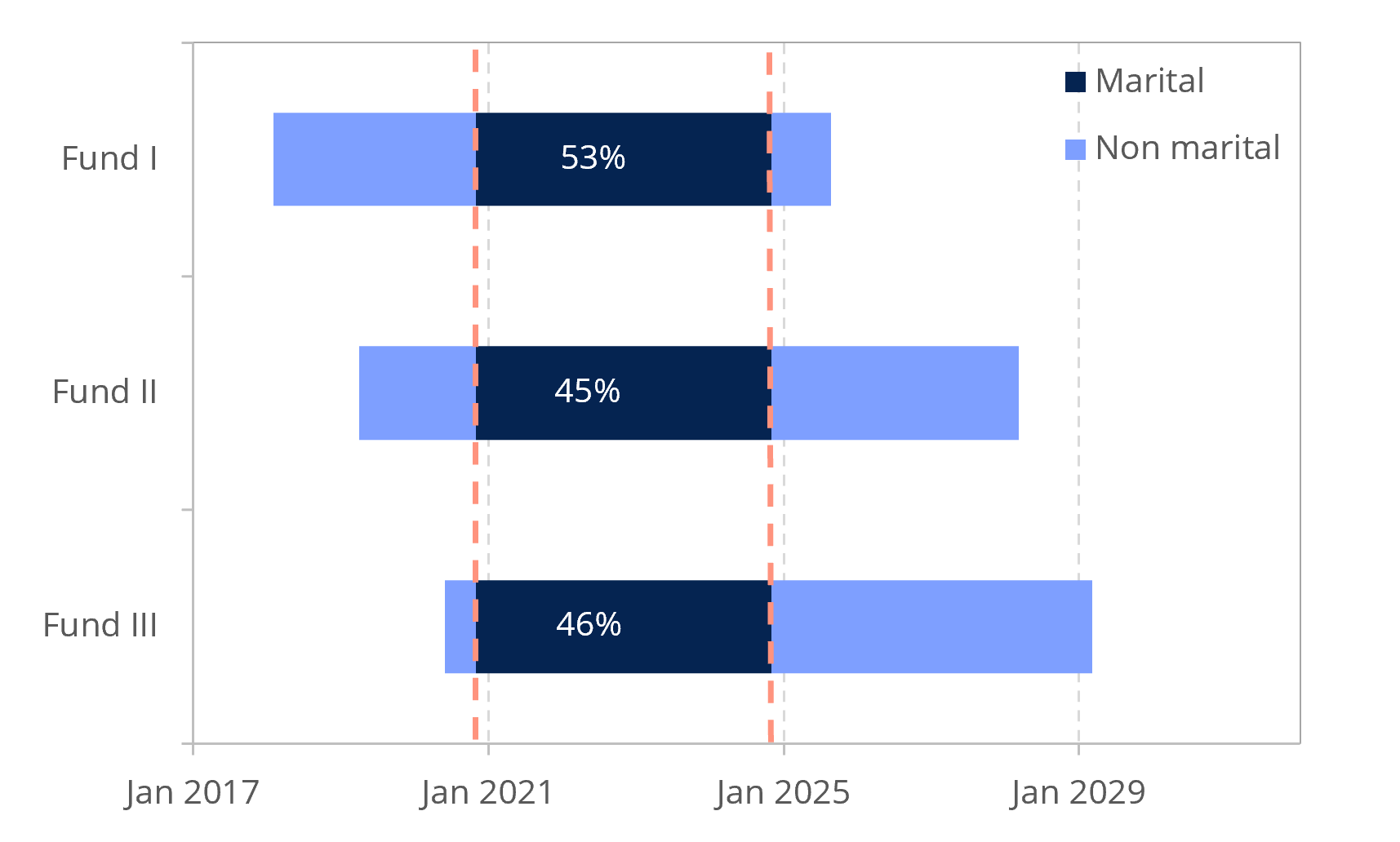
Figure 2: Illustrative example of the marital portion of Carry for funds which start before and end after the marriage. Dashed orange lines indicate the start and end of ‘A’ (the marital period)

(3) End date of ‘A’: in A v M (at [15]), Mostyn J considers that the marital period, ‘A’, should end on the date of the final hearing. Whilst not unreasonable, as with many other cases, we appreciate that there may be arguments for why date of separation is more appropriate. One for the lawyers, we are afraid!

(4) End date of ‘B’: in A v M (at [15]), Mostyn J considers that ‘B’ should represent the full lifetime of the Fund. However, as we explain above, under the A v M (Extended) approach, we consider it more consistent to adopt an end date of ‘B’ equal to the day that Carry is received (or receivable) by the relevant individual (which is of course unknown as at the date of final hearing). This is because once an investment is sold by the Fund and Carry is paid to the Carry Owner, it may be that little to no further work is required by the Carry Owner in respect of this investment even though the Fund itself may still continue its ‘lifetime’ for some (potentially considerable) period of time.

(5) Linear apportionment of work: as we discuss above, in ED v AP (at [58(v)]), HHJ Hess explains that it is not always appropriate to assume that work occurs linearly across the lifetime of the Fund. In our experience, significant work can be required throughout the lifetime of a Fund in respect of: (a) fundraising; (b) identifying investments; (c) completing acquisitions and performing the associated due diligence; (d) managing the acquired companies; and (e) completing sales and performing the associated due diligence. This may support adopting a ‘broad brush’ approach that Carry should be apportioned linearly. Equally, however, there will be specific cases where a linear approach may be inappropriate, depending on the facts of the case. In these instances, it may be that the A v M Formula can be suitably adjusted to apply additional weighting during the periods in which the Carry Owner undertakes significant work, with comparatively less weight applied during periods of less work. In practice, such an approach will be more mechanically complex and specialist advice may be required, for example, if a non-linear or weighted average approach is to be adopted when adjusting the A v M Formula to reflect alternative apportionments of work.

To assist, we have prepared a simplified Microsoft Excel spreadsheet, the ‘Illustrative A v M Calculator (RDA)’, alongside this article.[[3]] This allows the user to input various assumptions, as discussed above, including, importantly: (1) the date of actual Carry receipt in order to allow the sharing percentage under the A v M (Extended) method to be calculated, as based on the A v M Formula; and (2) the amount of actual Carry receipt so the shares in absolute terms can be ascertained.

Of course, both the inputs into the calculator (either as agreed by the parties or as determined by the court) and how the later receipt, when crystallised, is to be paid by the Carry Owner will need careful drafting. As accountants, it is not for us to comment on how an order should be drafted, but it will need to record in an appropriate way how the amount due to the Non Carry Owner should be calculated in the future (when all information is known). For example, it may include something along the lines of ‘the Non Carry Owner is to receive by way of deferred payment half of X% of the Carry Owner’s receipt due to their carry entitlement in fund Y, where X = A/B’ (with A and B then subject to bespoke definitions that can incorporate the actual date(s) of receipt).

Likewise, the amount of the receipt (including how any tax payable is to be accounted for) will need to be carefully drafted and consideration will also need to be given as to whether (and to what extent) there is a requirement for ongoing financial disclosure and/or security pending payment. However, we understand that these drafting and other considerations often (if not always) arise in Wells sharing cases, but we will (again) leave that to the lawyers!

Conclusion

In cases where Carry is to be Wells shared, we consider that a flexible, yet formulaic, approach, that builds on the strength of analysis put forward by both Mostyn J and HHJ Hess in A v M and ED v AP, respectively, to assess the marital proportion of Carry as at the date of its receipt, when all information is known, is both more consistent and reliable, as compared to fixing the sharing percentage in advance at a given point in time, based on uncertain and unknowable assumptions at the point of final hearing.

In our view, the A v M (Extended) method, as outlined in this article, provides a greater deal of flexibility and increases the scope for fairer outcomes, especially in circumstances where all assumptions can be agreed between the parties. It allows for a simple calculation to determine the marital proportion once Carry is received and hopefully reduces the scope for further dispute when issues of Carry arise in a case.